前置知识
如果我们在提到扩散模型就不能放过它的两个前置的知识:非平衡热力学和马尔可夫链
非平衡热力学
这是一种宏观上的确定性与微观上的随机性的结合,而整体的表现形式就好比把墨水滴入水中:
非平衡态:刚开始墨水和水分界明显(高浓度差),墨水分子剧烈扩散
平衡态:几小时后墨水均匀分布(浓度差消失),系统进入静止状态
非平衡热力学就是研究墨水扩散过程中的规律
核心矛盾:系统总在追求平衡(熵增原理),但外界干扰会打破平衡
典型特征:存在能量/物质流动(如扩散中的分子运动)
数学描述:用扩散方程等偏微分方程刻画浓度梯度与扩散速度的关系
代码例子
import pygame
import random
import sys
import math

# 初始化Pygame
pygame.init()
WIDTH, HEIGHT = 800, 600
screen = pygame.display.set_mode((WIDTH, HEIGHT))
pygame.display.set_caption("非平衡热力学扩散模型")

# 物理参数
LEFT_TEMP = 1.0  # 左侧初始温度
RIGHT_TEMP = 0.2  # 右侧初始温度
DRIFT_COEFF = 0.8  # 热泳效应漂移系数
DIFFUSION_BASE = 10  # 基础扩散系数

# 可视化参数
BACKGROUND_GRADIENT = []  # 预计算背景温度梯度


def create_gradient():
    """创建温度梯度背景"""
    for x in range(WIDTH):
        temp = LEFT_TEMP - (LEFT_TEMP - RIGHT_TEMP) * (x / WIDTH)
        color = (255 * temp, 0, 255 * (1 - temp))
        BACKGROUND_GRADIENT.append(color)


create_gradient()


class ThermodynamicParticle:
    def __init__(self):
        self.reset()

    def reset(self):
        """重置粒子到左侧随机位置"""
        self.x = random.uniform(0, WIDTH * 0.2)
        self.y = random.uniform(0, HEIGHT)
        self.history = [(self.x, self.y)] * 5  # 轨迹存储

    @property
    def temperature(self):
        """根据位置计算温度"""
        return LEFT_TEMP - (LEFT_TEMP - RIGHT_TEMP) * (self.x / WIDTH)

    def update(self):
        """更新粒子运动状态"""
        # 计算温度相关参数
        temp = self.temperature
        drift = DRIFT_COEFF * (1 + math.sin(self.x / 50))  # 带波动性的漂移
        diffusion = DIFFUSION_BASE * temp

        # 更新位置(漂移+扩散+噪声)
        self.x += drift + random.uniform(-diffusion, diffusion)
        self.y += random.uniform(-diffusion, diffusion) * 0.5 + random.gauss(0, 0.5)

        # 边界处理
        if self.x > WIDTH * 0.95:  # 右侧粒子重置
            self.reset()
        self.x = max(0, min(self.x, WIDTH))
        self.y = max(0, min(self.y, HEIGHT))

        # 更新轨迹
        self.history.pop(0)
        self.history.append((self.x, self.y))

    def draw(self, surface):
        """绘制粒子和运动轨迹"""
        # 绘制运动轨迹
        for i, pos in enumerate(self.history):
            alpha = 50 + 40 * i
            pygame.draw.circle(surface, (255, 255, 255, alpha), pos, i // 2)

        # 绘制当前粒子
        color = (255 * self.temperature, 150, 255 * (1 - self.temperature))
        pygame.draw.circle(surface, color, (int(self.x), int(self.y)), 3)


# 初始化粒子系统
particles = [ThermodynamicParticle() for _ in range(300)]

# 主循环
clock = pygame.time.Clock()
running = True

while running:
    # 事件处理
    for event in pygame.event.get():
        if event.type == pygame.QUIT:
            running = False

    # 绘制温度梯度背景
    for x in range(WIDTH):
        pygame.draw.line(screen, BACKGROUND_GRADIENT[x], (x, 0), (x, HEIGHT))

    # 更新并绘制粒子
    for p in particles:
        p.update()
        p.draw(screen)

    # 显示状态信息
    fps = clock.get_fps()
    pygame.display.set_caption(f"非平衡热力学扩散模型 | 粒子数: {len(particles)} | FPS: {fps:.1f}")
    pygame.display.flip()
    clock.tick(60)

pygame.quit()
sys.exit()
关键特性说明
背景颜色从左到右呈现红→蓝渐变,直观显示温度分布
粒子颜色根据当前位置温度变化(红→蓝)
热泳效应驱动粒子从高温区向低温区迁移
温度依赖的扩散系数(高温区扩散更剧烈)
右侧边界重置机制维持系统非平衡状态

与扩散模型的联系
比如在一个生成式的扩散模型中
前向过程(破坏数据):图像 ➔ 逐步加噪 ➔ 随机噪声 (模拟非平衡态熵增)
逆向过程(生成数据):随机噪声 ➔ 逐步去噪 ➔ 清晰图像 (模拟逆熵过程)加噪:类似墨水扩散,通过马尔可夫链逐步破坏数据结构
去噪:需要神经网络预测每个步骤的噪声(相当于重建浓度梯度)
马尔可夫链
马尔科夫链是一种具有无记忆性质的随机过程,其中下一状态仅依赖于当前状态,而与之前的状态无关。其核心要素是状态空间与转移概率矩阵
假设天气只有两种状态:晴天和雨天
如果今天是晴天,明天有80%概率仍是晴天,20%概率下雨。
如果今天下雨,明天有60%概率转晴,40%概率继续下雨。
代码例子
import random

# 定义状态和转移概率矩阵
states = ['Sunny', 'Rainy']
transition_matrix = {
    'Sunny': {'Sunny': 0.8, 'Rainy': 0.2},
    'Rainy': {'Sunny': 0.6, 'Rainy': 0.4}
}

# 模拟马尔科夫链
current_state = 'Sunny'
chain = [current_state]

for _ in range(5):  # 模拟5步
    next_states = list(transition_matrix[current_state].keys())
    weights = list(transition_matrix[current_state].values())
    current_state = random.choices(next_states, weights=weights)[0]
    chain.append(current_state)

print("模拟路径(字典方法):", chain)
在扩散模型中的应用
扩散模型通过神经网络学习复杂的生成规则,且需要多步逆向去噪。马尔科夫链在扩散模型中“给神经网络制造困难”,正向扩散过程通过逐步添加噪声破坏数据从而构造一个可逆的概率路径,使神经网络能够学习从噪声中恢复原始数据的规律。正因为如此扩散模型属于一种典型的无监督学习又可以叫自监督学习
扩散模型
核心框架
正向扩散过程(加噪)
将一张真实图片通过多步(通常数百至数千步)逐渐添加高斯噪声,最终转化为纯噪声。这一过程满足马尔科夫链性质,即每一步仅依赖前一步的状态。
这里使用Python做一个演示
import numpy as np
from PIL import Image
import matplotlib.pyplot as plt
def markov_chain_noise(image_path, steps=5, beta_start=0.01, beta_end=0.5):
"""
马尔科夫链逐步加噪演示
:param image_path: 输入图片路径
:param steps: 加噪步数
:param beta_start: 初始噪声系数
:param beta_end: 最终噪声系数
:return: 各步骤噪声图像列表
"""
orig_image = Image.open(image_path)
image_array = np.array(orig_image) / 255.0 # 归一化到[0,1]
betas = np.linspace(beta_start, beta_end, steps)
noisy_images = [orig_image]
x = image_array.copy()
for t in range(steps):
noise = np.random.normal(size=image_array.shape)
beta_t = betas[t]
x = np.sqrt(1 - beta_t) * x + np.sqrt(beta_t) * noise
noisy_img = Image.fromarray(
(np.clip(x, 0, 1) * 255).astype(np.uint8)
)
noisy_images.append(noisy_img)
return noisy_images
if __name__ == "__main__":
input_image = r"你的图片位置"
total_steps = 6
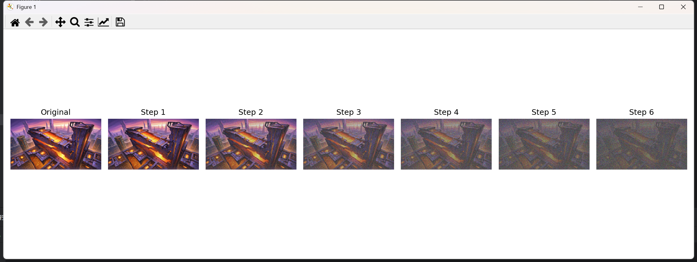
results = markov_chain_noise(input_image, steps=total_steps)
plt.figure(figsize=(15, 5))
for i, img in enumerate(results):
plt.subplot(1, len(results), i + 1)
plt.imshow(img)
plt.title(f"Step {i}" if i > 0 else "Original")
plt.axis('off')
plt.tight_layout()
plt.savefig("noise_progression.png")
plt.show()反向去噪过程(生成)
训练神经网络从纯噪声开始,逐步预测并去除噪声,最终复原出原始图像的结构。这一逆过程同样遵循马尔科夫链的逐步推导。
训练流程
我们以单张图像举例子,目标图像为

数据预处理阶段
加载128x128灰度目标图像
应用标准化处理(归一化到[-1,1]范围)
转换为PyTorch张量并添加批次维度
存储在GPU显存中
模型架构构建
改进型UNet结构包含:
正弦位置编码(SinusoidalPositionEmbeddings)
4级下采样模块(通道数64→128→256→512)
1个瓶颈层
3级上采样模块(含跳跃连接)
时间步信息通过线性层注入每个Block
使用GroupNorm归一化和SiLU激活函数
最终输出层为1x1卷积
扩散参数初始化
总扩散步数T=1000
采用余弦调度生成beta序列:
使用cos^2曲线生成alpha累积乘积
推导得到beta值范围[0.0001, 0.02]
预计算存储:
α = 1 - β
α_bar = ∏α (累积乘积)
训练循环
随机采样时间步
生成0到999之间的随机整数
前向扩散过程
生成标准正态分布噪声ε ~ N(0,I)
计算当前步的α_bar值
合成加噪图像:x_t = sqrt(α_{bar})*x_0 + sqrt(1-α_{bar})*ε
噪声预测
将加噪图像和时间步t输入UNet
模型输出预测噪声ε_θ
损失计算与优化
计算预测噪声与真实噪声的MSE损失
梯度清零
反向传播计算梯度
梯度裁剪(最大范数1.0)
AdamW优化器更新参数
余弦退火学习率调度(周期1000步)
图像生成阶段
初始化
生成128x128标准正态分布噪声
设置生成步数steps=1000
确定性系数eta=0
逆向扩散过程
这是一个从999到0的递减循环
预测当前噪声ε_θ
估计初始图像x_0_pred
计算前步的α_bar值
根据DDIM公式更新x:x_{t-1} = \sqrt{\bar{\alpha}_{t-1}} \hat{x}_0 + \sqrt{1 - \bar{\alpha}_{t-1} - \sigma^2} \epsilon_\theta + \sigma \tilde{\varepsilon}
最后一步(t=0)时不添加随机噪声
后处理
将输出值截断到[-1,1]范围
线性映射到[0,1]区间
移除批次维度,返回CPU张量
最终结果
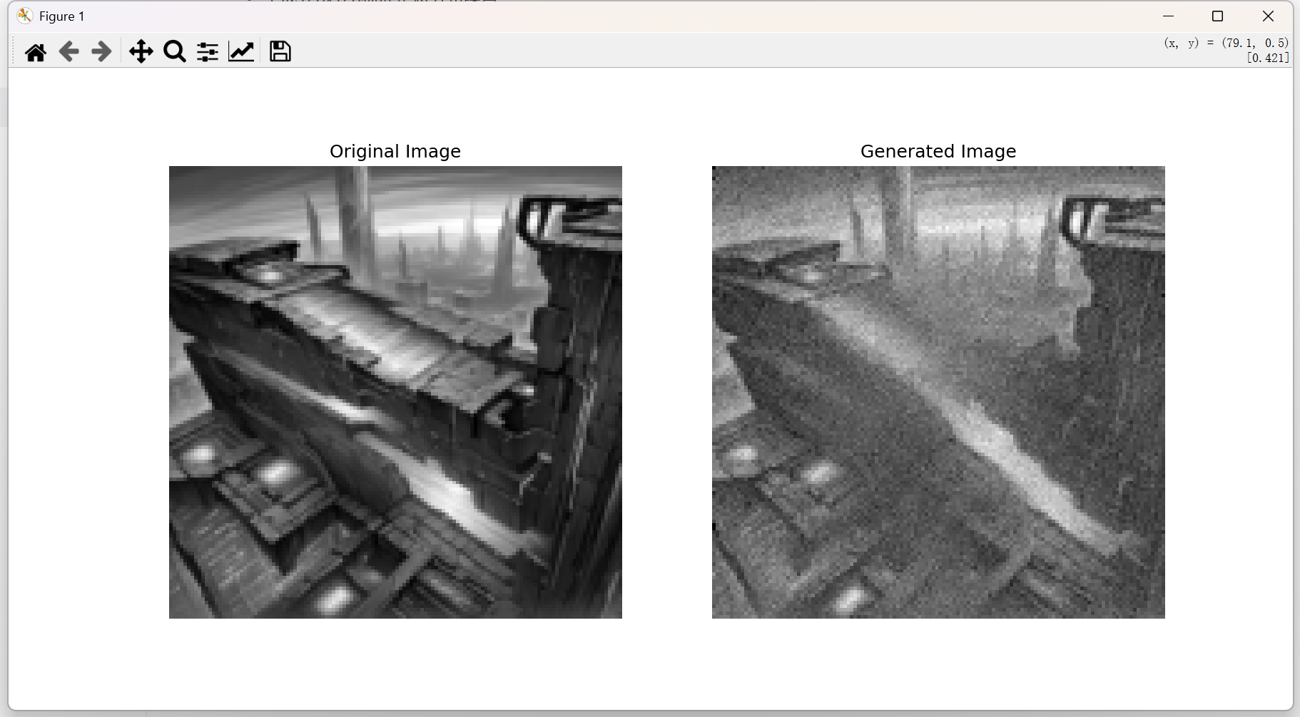
这是迭代了150000次的结果
参数
| 超参数类别 | 参数名称 | 设置值 | 说明 |
|---|---|---|---|
| 模型架构 | |||
| 模型架构 | time_emb_dim | 32 | 时间步嵌入的维度数 |
| 模型架构 | GroupNorm groups | 8 | 归一化层的分组数量 |
| 扩散过程 | |||
| 扩散过程 | T | 1000 | 前向扩散总步数 |
| 扩散过程 | s | 0.008 | 余弦偏移系数 |
| 训练设置 | |||
| 训练设置 | epochs | 15,000 | 总训练轮次 |
| 训练设置 | batch_size | 1 | 单样本训练 |
| 优化器 | |||
| 优化器 | Learning rate | 2e-4 | 初始学习率 |
| 优化器 | grad_clip | 1.0 | 梯度最大范数限制 |
| 生成参数 | |||
| 生成参数 | steps | 1000 | 逆向扩散总步数 |
| 生成参数 | img_size | 128x128 | 生成图像分辨率 |
完整代码
这里使用torch,需要提前安装好torch
import torch
import torch.nn as nn
import torch.optim as optim
from torchvision import transforms
from PIL import Image
import matplotlib.pyplot as plt
import math

# ========== 设备配置 ==========
device = torch.device("cuda" if torch.cuda.is_available() else "cpu")


# ========== 数据预处理 ==========
def load_image(path, img_size=128):
    transform = transforms.Compose([
        transforms.Resize(img_size),
        transforms.CenterCrop(img_size),
        transforms.ToTensor(),
        transforms.Normalize([0.5], [0.5])
    ])
    image = Image.open(path).convert('L')
    return transform(image).unsqueeze(0).to(device)


target_img = load_image(r"目标图片地址写进这里")


# ========== 改进的UNet模型 ==========
class Block(nn.Module):
    def __init__(self, in_ch, out_ch, time_emb_dim):
        super().__init__()
        self.time_mlp = nn.Linear(time_emb_dim, out_ch)
        self.conv1 = nn.Conv2d(in_ch, out_ch, 3, padding=1)
        self.conv2 = nn.Conv2d(out_ch, out_ch, 3, padding=1)
        self.norm = nn.GroupNorm(8, out_ch)
        self.act = nn.SiLU()

    def forward(self, x, t):
        h = self.norm(self.conv1(x))
        h += self.time_mlp(t)[:, :, None, None]
        h = self.act(h)
        h = self.norm(self.conv2(h))
        h = self.act(h)
        return h


class ImprovedUNet(nn.Module):
    def __init__(self):
        super().__init__()
        self.time_emb_dim = 32
        self.time_mlp = nn.Sequential(
            SinusoidalPositionEmbeddings(self.time_emb_dim),
            nn.Linear(self.time_emb_dim, self.time_emb_dim),
            nn.SiLU()
        )

        self.down1 = Block(1, 64, self.time_emb_dim)
        self.down2 = Block(64, 128, self.time_emb_dim)
        self.down3 = Block(128, 256, self.time_emb_dim)
        self.bottleneck = Block(256, 512, self.time_emb_dim)

        self.up1 = Block(512 + 256, 256, self.time_emb_dim)
        self.up2 = Block(256 + 128, 128, self.time_emb_dim)
        self.up3 = Block(128 + 64, 64, self.time_emb_dim)

        self.final_conv = nn.Conv2d(64, 1, 1)

    def forward(self, x, t):
        t_emb = self.time_mlp(t)

        # 下采样
        x1 = self.down1(x, t_emb)
        x2 = self.down2(nn.MaxPool2d(2)(x1), t_emb)
        x3 = self.down3(nn.MaxPool2d(2)(x2), t_emb)
        x4 = self.bottleneck(nn.MaxPool2d(2)(x3), t_emb)

        # 上采样
        x = nn.Upsample(scale_factor=2)(x4)
        x = self.up1(torch.cat([x, x3], dim=1), t_emb)
        x = nn.Upsample(scale_factor=2)(x)
        x = self.up2(torch.cat([x, x2], dim=1), t_emb)
        x = nn.Upsample(scale_factor=2)(x)
        x = self.up3(torch.cat([x, x1], dim=1), t_emb)

        return self.final_conv(x)


class SinusoidalPositionEmbeddings(nn.Module):
    def __init__(self, dim):
        super().__init__()
        self.dim = dim

    def forward(self, time):
        device = time.device
        half_dim = self.dim // 2
        embeddings = math.log(10000) / (half_dim - 1)
        embeddings = torch.exp(torch.arange(half_dim, device=device) * -embeddings)
        embeddings = time[:, None] * embeddings[None, :]
        embeddings = torch.cat((embeddings.sin(), embeddings.cos()), dim=-1)
        return embeddings


# ========== 扩散参数设置 ==========
T = 1000
beta_start = 0.0001
beta_end = 0.02


# 使用余弦调度
def cosine_beta_schedule(timesteps):
    s = 0.008
    steps = timesteps + 1
    x = torch.linspace(0, timesteps, steps)
    alphas_cumprod = torch.cos(((x / timesteps) + s) / (1 + s) * math.pi * 0.5) ** 2
    alphas_cumprod = alphas_cumprod / alphas_cumprod[0]
    betas = 1 - (alphas_cumprod[1:] / alphas_cumprod[:-1])
    return torch.clamp(betas, 0.0001, 0.02)


betas = cosine_beta_schedule(T).to(device)
alphas = 1 - betas
alpha_bars = torch.cumprod(alphas, dim=0)

# ========== 模型初始化 ==========
model = ImprovedUNet().to(device)
optimizer = optim.AdamW(model.parameters(), lr=2e-4)
scheduler = optim.lr_scheduler.CosineAnnealingLR(optimizer, T_max=1000)
criterion = nn.MSELoss()

# ========== 训练循环 ==========
for epoch in range(15000):
    t = torch.randint(0, T, (1,)).long().to(device)

    # 前向扩散
    noise = torch.randn_like(target_img)
    alpha_bar = alpha_bars[t].view(-1, 1, 1, 1)
    noisy_img = torch.sqrt(alpha_bar) * target_img + torch.sqrt(1 - alpha_bar) * noise

    # 噪声预测
    pred_noise = model(noisy_img, t)

    # 反向传播
    loss = criterion(pred_noise, noise)
    optimizer.zero_grad()
    loss.backward()
    torch.nn.utils.clip_grad_norm_(model.parameters(), 1.0)
    optimizer.step()
    scheduler.step()

    if epoch % 100 == 0:
        print(f"Epoch {epoch}, Loss: {loss.item():.4f}")


# ========== 改进的图像生成 ==========
@torch.no_grad()
def generate(num_samples=1, steps=T, eta=0.0):
    model.eval()
    x = torch.randn((num_samples, 1, 128, 128), device=device)

    for t in reversed(range(0, steps)):
        t_batch = torch.full((num_samples,), t, device=device, dtype=torch.long)
        pred_noise = model(x, t_batch)

        alpha_bar_t = alpha_bars[t]
        alpha_bar_t_prev = alpha_bars[t - 1] if t > 0 else torch.tensor(1.0, device=device)  # 修改这里

        # DDIM推导公式
        pred_x0 = (x - torch.sqrt(1 - alpha_bar_t) * pred_noise) / torch.sqrt(alpha_bar_t)

        sigma = eta * torch.sqrt((1 - alpha_bar_t_prev) / (1 - alpha_bar_t) * (1 - alpha_bar_t / alpha_bar_t_prev))

        epsilon = torch.randn_like(x) if t > 0 else torch.zeros_like(x)  # 修改这里

        x = torch.sqrt(alpha_bar_t_prev) * pred_x0 + \
            torch.sqrt(1 - alpha_bar_t_prev - sigma ** 2) * pred_noise + \
            sigma * epsilon

    generated = (x.clamp(-1, 1) + 1) / 2
    return generated.cpu().squeeze()


# ========== 结果可视化 ==========
plt.figure(figsize=(12, 6))
plt.subplot(121)
plt.imshow(target_img.cpu().squeeze(), cmap='gray')
plt.title('Original Image')
plt.axis('off')

plt.subplot(122)
plt.imshow(generate(eta=0.0), cmap='gray')  # 使用DDIM采样
plt.title('Generated Image')
plt.axis('off')
plt.show()